Using H2O AutoML
Automatic machine learning (AutoML) is the process of automatically
searching, screening and evaluating many models for a specific dataset.
AutoML could be particularly insightful as an exploratory approach to
identify model families and parameterization that is most likely to
succeed. You can use H2O’s AutoML
algorithm via the 'h2o' engine in auto_ml().
agua provides several helper functions to quickly wrangle and visualize
AutoML’s results.
Let’s run an AutoML search on the concrete data.
library(tidymodels)
library(agua)
library(ggplot2)
theme_set(theme_bw())
h2o_start()
#> Warning: JAVA not found, H2O may take minutes trying to connect.
#> Warning in h2o.clusterInfo():
#> Your H2O cluster version is (5 months and 15 days) old. There may be a newer version available.
#> Please download and install the latest version from: https://h2o-release.s3.amazonaws.com/h2o/latest_stable.html
data(concrete)
set.seed(4595)
concrete_split <- initial_split(concrete, strata = compressive_strength)
concrete_train <- training(concrete_split)
concrete_test <- testing(concrete_split)

# run for a maximum of 120 seconds
auto_spec <-
  auto_ml() %>%
  set_engine("h2o", max_runtime_secs = 120, seed = 1) %>%
  set_mode("regression")

normalized_rec <-
  recipe(compressive_strength ~ ., data = concrete_train) %>%
  step_normalize(all_predictors())

auto_wflow <-
  workflow() %>%
  add_model(auto_spec) %>%
  add_recipe(normalized_rec)

auto_fit <- fit(auto_wflow, data = concrete_train)
#> Warning in use.package("data.table"): data.table cannot be used without R
#> package bit64 version 0.9.7 or higher.  Please upgrade to take advangage
#> of data.table speedups.
extract_fit_parsnip(auto_fit)
#> parsnip model object
#>
#> ═════════════════════ H2O AutoML Summary: 105 models ═════════════════════
#>
#>
#> ═══════════════════════════════ Leaderboard ══════════════════════════════
#>                                                 model_id rmse  mse  mae
#> 1 StackedEnsemble_BestOfFamily_4_AutoML_1_20240605_21232 4.51 20.4 3.00
#> 2    StackedEnsemble_AllModels_2_AutoML_1_20240605_21232 4.62 21.4 3.04
#> 3    StackedEnsemble_AllModels_1_AutoML_1_20240605_21232 4.67 21.8 3.08
#> 4 StackedEnsemble_BestOfFamily_3_AutoML_1_20240605_21232 4.68 21.9 3.08
#> 5 StackedEnsemble_BestOfFamily_2_AutoML_1_20240605_21232 4.71 22.2 3.16
#> 6                          GBM_5_AutoML_1_20240605_21232 4.75 22.6 3.14
#>   rmsle mean_residual_deviance
#> 1 0.141                   20.4
#> 2 0.140                   21.4
#> 3 0.142                   21.8
#> 4 0.142                   21.9
#> 5 0.146                   22.2
#> 6 0.147                   22.6
In 120 seconds, AutoML fitted 105 models. The parsnip fit object
extract_fit_parsnip(auto_fit) shows the number of candidate
models, the best performing algorithm and its corresponding model id,
and a preview of the leaderboard with cross validation performances. The
model_id column in the leaderboard is a unique model
identifier for the h2o server. This can be useful when you need to
predict on or extract a specific model, e.g. with
predict(auto_fit, id = id) and
extract_fit_engine(auto_fit, id = id). By default, they
will operate on the best performing leader model.
# predict with the best model
predict(auto_fit, new_data = concrete_test)
#> Warning in use.package("data.table"): data.table cannot be used without R
#> package bit64 version 0.9.7 or higher.  Please upgrade to take advangage
#> of data.table speedups.
#> # A tibble: 260 × 1
#>    .pred
#>    <dbl>
#>  1  40.0
#>  2  43.0
#>  3  38.2
#>  4  55.7
#>  5  41.4
#>  6  28.1
#>  7  53.2
#>  8  34.5
#>  9  51.1
#> 10  37.9
#> # ℹ 250 more rows
Typically, we use AutoML to get a quick sense of the range of our success metric, and algorithms that are likely to succeed. agua provides tools to summarize these results.
-
rank_results()returns the leaderboard in a tidy format with rankings within each metric. A low rank means good performance in a metric. Here, the top 5 models with the smallest MAE includes are four stacked ensembles and one GBM model.
rank_results(auto_fit) %>%
  filter(.metric == "mae") %>%
  arrange(rank)
#> # A tibble: 105 × 5
#>    id                                        algorithm .metric  mean  rank
#>    <chr>                                     <chr>     <chr>   <dbl> <int>
#>  1 StackedEnsemble_BestOfFamily_4_AutoML_1_… stacking  mae      3.00     1
#>  2 StackedEnsemble_AllModels_2_AutoML_1_202… stacking  mae      3.04     2
#>  3 StackedEnsemble_BestOfFamily_3_AutoML_1_… stacking  mae      3.08     3
#>  4 StackedEnsemble_AllModels_1_AutoML_1_202… stacking  mae      3.09     4
#>  5 XGBoost_grid_1_AutoML_1_20240605_21232_m… xgboost   mae      3.13     5
#>  6 XGBoost_grid_1_AutoML_1_20240605_21232_m… xgboost   mae      3.14     6
#>  7 GBM_5_AutoML_1_20240605_21232             gradient… mae      3.15     7
#>  8 StackedEnsemble_BestOfFamily_2_AutoML_1_… stacking  mae      3.17     8
#>  9 XGBoost_grid_1_AutoML_1_20240605_21232_m… xgboost   mae      3.18     9
#> 10 GBM_grid_1_AutoML_1_20240605_21232_model… gradient… mae      3.18    10
#> # ℹ 95 more rows-
collect_metrics()returns average statistics of performance metrics (summarized) per model, or raw value for each resample (unsummarized).cv_ididentifies the resample h2o internally used for optimization.
collect_metrics(auto_fit, summarize = FALSE)
#> # A tibble: 3,720 × 5
#>    id                                    algorithm .metric cv_id .estimate
#>    <chr>                                 <chr>     <chr>   <chr>     <dbl>
#>  1 StackedEnsemble_BestOfFamily_4_AutoM… stacking  mae     cv_1…      2.81
#>  2 StackedEnsemble_BestOfFamily_4_AutoM… stacking  mae     cv_2…      2.92
#>  3 StackedEnsemble_BestOfFamily_4_AutoM… stacking  mae     cv_3…      2.83
#>  4 StackedEnsemble_BestOfFamily_4_AutoM… stacking  mae     cv_4…      3.41
#>  5 StackedEnsemble_BestOfFamily_4_AutoM… stacking  mae     cv_5…      3.02
#>  6 StackedEnsemble_BestOfFamily_4_AutoM… stacking  mean_r… cv_1…     17.7
#>  7 StackedEnsemble_BestOfFamily_4_AutoM… stacking  mean_r… cv_2…     20.5
#>  8 StackedEnsemble_BestOfFamily_4_AutoM… stacking  mean_r… cv_3…     16.9
#>  9 StackedEnsemble_BestOfFamily_4_AutoM… stacking  mean_r… cv_4…     27.6
#> 10 StackedEnsemble_BestOfFamily_4_AutoM… stacking  mean_r… cv_5…     19.1
#> # ℹ 3,710 more rows-
tidy()returns a tibble with performance and individual model objects. This is helpful if you want to perform operations (e.g., predict) across all candidates.
tidy(auto_fit) %>%
  mutate(
    .predictions = map(.model, predict, new_data = head(concrete_test))
  )
#> Warning: There were 105 warnings in `mutate()`.
#> The first warning was:
#> ℹ In argument: `.predictions = map(.model, predict, new_data =
#>   head(concrete_test))`.
#> Caused by warning in `use.package()`:
#> ! data.table cannot be used without R package bit64 version 0.9.7 or higher.  Please upgrade to take advangage of data.table speedups.
#> ℹ Run `dplyr::last_dplyr_warnings()` to see the 104 remaining warnings.
#> # A tibble: 105 × 5
#>    id                             algorithm .metric  .model   .predictions
#>    <chr>                          <chr>     <list>   <list>   <list>
#>  1 StackedEnsemble_BestOfFamily_… stacking  <tibble> <fit[+]> <tibble>
#>  2 StackedEnsemble_AllModels_2_A… stacking  <tibble> <fit[+]> <tibble>
#>  3 StackedEnsemble_AllModels_1_A… stacking  <tibble> <fit[+]> <tibble>
#>  4 StackedEnsemble_BestOfFamily_… stacking  <tibble> <fit[+]> <tibble>
#>  5 StackedEnsemble_BestOfFamily_… stacking  <tibble> <fit[+]> <tibble>
#>  6 GBM_5_AutoML_1_20240605_21232  gradient… <tibble> <fit[+]> <tibble>
#>  7 GBM_grid_1_AutoML_1_20240605_… gradient… <tibble> <fit[+]> <tibble>
#>  8 XGBoost_grid_1_AutoML_1_20240… xgboost   <tibble> <fit[+]> <tibble>
#>  9 XGBoost_grid_1_AutoML_1_20240… xgboost   <tibble> <fit[+]> <tibble>
#> 10 GBM_3_AutoML_1_20240605_21232  gradient… <tibble> <fit[+]> <tibble>
#> # ℹ 95 more rows-
member_weights()computes member importance for all stacked ensemble models. Aside from base models such as GLM, GBM and neural networks, h2o tries to fit two kinds of stacked ensembles: one combines all the base models ("all") and the other includes only the best model of each kind ("bestofFamily"), specific to a time point. Regardless of how ensembles are formed, we can calculate the variable importance in the ensemble as the importance score of every member model, i.e., the relative contribution of base models in the meta-learner. This is typically the coefficient magnitude in a second-level GLM. This way, in addition to inspecting model performances by themselves, we can find promising candidates if stacking is needed. Here, we show the scaled contribution of different algorithms in stacked ensembles.
auto_fit %>%
  extract_fit_parsnip() %>%
  member_weights() %>%
  unnest(importance) %>%
  filter(type == "scaled_importance") %>%
  ggplot() +
  geom_boxplot(aes(value, algorithm)) +
  scale_x_sqrt() +
  labs(y = NULL, x = "scaled importance", title = "Member importance in stacked ensembles")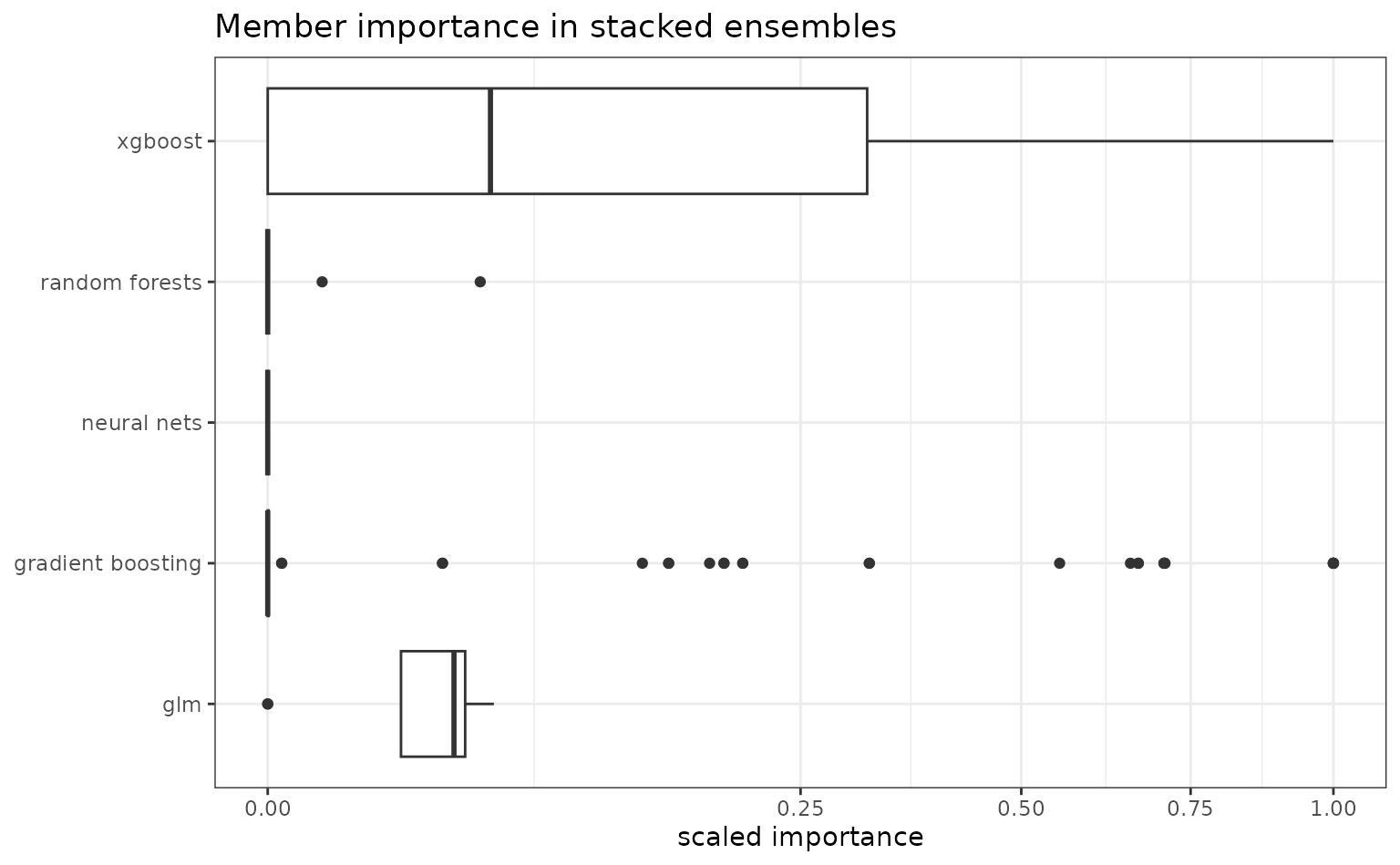
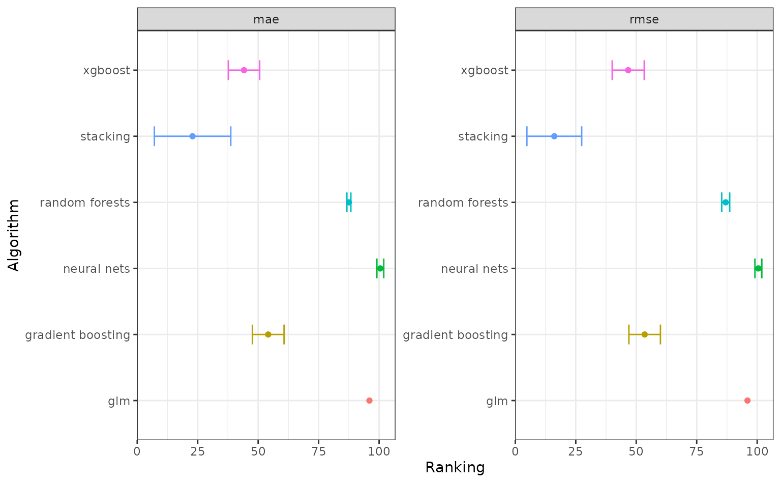
You can also autoplot() an AutoML object, which
essentially wraps functions above to plot performance assessment and
ranking. The lower the average ranking, the more likely the model type
suits the data.
After initial assessment, we might be interested to allow more time
for AutoML to search for more candidates. Recall that we have set engine
argument max_runtime_secs to 120s before, we can increase
it or adjust max_models to control the total runtime. H2O
also provides an option to build upon an existing AutoML leaderboard and
add more candidates, this can be done via refit(). The
model to be re-fitted needs to have engine argument
save_data = TRUE. If you also want to add stacked ensembles
set keep_cross_validation_predictions = TRUE as well.
# not run
auto_spec_refit <-
  auto_ml() %>%
  set_engine("h2o",
             max_runtime_secs = 300,
             save_data = TRUE,
             keep_cross_validation_predictions = TRUE) %>%
  set_mode("regression")

auto_wflow_refit <-
  workflow() %>%
  add_model(auto_spec_refit) %>%
  add_recipe(normalized_rec)

first_auto <- fit(auto_wflow_refit, data = concrete_train)
# fit another 60 seconds
second_auto <- refit(first_auto, max_runtime_secs = 60)
Important engine arguments
There are several relevant engine arguments for H2O AutoML, some of the most commonly used are:
max_runtime_secsandmax_models: Adjust runtime.include_algosandexclude_algos: A character vector naming the algorithms to include or exclude.validation: An integer between 0 and 1 specifying the proportion of training data reserved as validation set. This is used by h2o for performance assessment and potential early stopping.
See the details section in h2o::h2o.automl() for more
information.